Understanding UI Layout Constraints (part 1)
This is the first in a series of posts where I attempt to understand and explain how UI layout constraints (such as Apple's Auto Layout) work and are implemented. Along the way, we will learn about a field of mathematics known as "linear programming".
In this first post, I will introduce the concepts of UI layout constraints and linear programming. I will also convert a UI layout constraint example into a system of linear equations, and graph the system visually. In future posts, I will explain the simplex method, the Cassowary algorithm, and how to implement the Cassowary algorithm as a computer program.
This series is mainly targeted at software developers who want to understand how UI layout constraint algorithms work, but who don't necessarily have a very strong or recent background in mathematics. I will assume you are familiar with basic algebra such as y ≤ 2x + 3. More advanced concepts will be explained as they are used.
Please be advised that I am not an expert on linear programming or these algorithms. I'm just a software developer who got curious. I will try to explain things as clearly and accurately as I can, but I might make some mistakes. If you have any questions, comments, feedback, or corrections, please email me: john (at) croisant (dot) net.
If you find this series interesting, enjoyable, or useful, please send me a little email to let me know. I spent a long time researching, writing, and polishing this series. It's nice to hear that my efforts have made a positive difference (however small) in someone else's life.
Update history:
- 2016-05-01: Removed links to learning resources, and "Preparing for the Simplex Method" section; updated versions of them will appear in the next post in this series. Tweaked description of the objective function. Added "Recap" section.
Table of Contents
- Series Introduction and Motivation
- Choice of Algorithm
- UI Layout Constraints
- Linear Programming
- Expressing UI Layout Constraints as a Linear System
- Graphing the System
- Recap
Series Introduction and Motivation
Recently I became interested in UI layout constraints, such as Apple's Auto Layout. I wondered how they worked, and how they are implemented. My search led me to the Cassowary algorithm.
The Cassowary site suggests that Auto Layout is based on the Cassowary algorithm. This is certainly plausible, although I can't confirm it because Auto Layout is closed source and the docs don't say what algorithm it uses. But even if Auto Layout is not directly based on the Cassowary algorithm, they are very similar and share the same concepts, so understanding the Cassowary algorithm will help us understand how Auto Layout works.
The Cassowary algorithm is described in the paper, The Cassowary Linear Arithmetic Constraint Solving Algorithm (2002) by Greg J. Badros, Alan Borning, and Peter J. Stuckey. (There is an earlier 1998 paper, but the 2002 paper has essentially the same information, and is a bit more polished and approachable.)
Unfortunately, I do not have a strong background in mathematics, and the paper is full of symbols, terminology, and concepts I wasn't familiar with, so I found it very difficult to read and understand.
To help me understand the Cassowary algorithm, I needed to study linear programming and the simplex method, upon which the Cassowary algorithm is based. Every introductory linear programming textbook explains the simplex method, but I wasn't sure if I was interested enough in this topic to justify purchasing an expensive textbook. So I decided to first try learning via online resources.
Even after reading many online resources, I still didn't fully grasp the simplex method, let alone the Cassowary algorithm. When I am struggling to learn something, it usually helps if I try to write about it. Explaining the concept forces me to think more deeply about it, and fill in the missing pieces that I didn't understand yet. So, I decided to write this series primarily to help myself understand. Hopefully it will help you understand, too.
Choice of Algorithm
There are several algorithms that can be used to solve UI layout constraints and other linear programming problems. In this series, I will be focusing on the simplex method (the most well-known linear programming algorithm), as well as the Cassowary algorithm (which is based on the simplex method).
If you are a software developer interested in implementing a UI layout constraint solver (or other linear programming solver), please be aware that the original simplex method is not an efficient algorithm for a computer implementation. As Paul Khuong writes:
The problem is that simplex only works because world-class implementations are marvels of engineering: it's almost like their performance is in spite of the algorithm, only thanks to coder-centuries of effort. Worse, textbooks usually present the classic simplex method (the dark force behind simplex tableaux) so that's what unsuspecting hackers implement. Pretty much no one uses that method: it's slow and doesn't really exploit sparsity (the fact that each constraint tends to only involve a few variables).
Paul Khuong recommends a different linear programming algorithm, called the interior point method (IPM). IPM is more efficient than the simplex method in some use cases, but I am going to focus on learning the simplex method and the Cassowary algorithm, for several reasons:
- I am interested specifically in solving UI layout constraints, not other kinds of linear programming problems.
- The Cassowary algorithm was designed and optimized for the needs of real-time interactive constraints, especially UI layout constraints.
- The Cassowary algorithm is based on the simplex method, so I need to understand the simplex method before I can fully understand the Cassowary algorithm. (The Cassowary algorithm fixes the problems of the simplex method that Paul Khuong describes.)
If your purpose or circumstances are different than mine, you should probably also have a look at IPM and other linear programming algorithms. They might be simpler or perform better than the Cassowary algorithm for your use case.
UI Layout Constraints
In case you're not familiar with the concept, UI layout constraint systems allow you to specify requirements or preferences about how a computer program's user interface should be arranged. The computer then calculates how to lay out the UI so that all the constraints are satisfied. This makes it relatively easy for designers to create UIs that automatically adapt to different circumstances, such as different content and screen sizes.
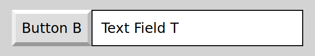
In this series, I will use a simple example involving two UI elements positioned side by side. One element is a button, which we will call B. The other is a text field, which we will call T. The type of UI element doesn't affect the algorithm or the result, I just wanted to make the example specific and easy to remember. Here is how our UI might be arranged:
Our goal is to figure out how wide B and T should be. Our example UI has the following specifications:
- Both elements should be as wide as possible, but it is most important for B to be as wide as possible.
- B must be at least 50 pixels wide.
- T must be at least twice as wide as B.
- Both elements side by side must fit in a 300 pixel wide area.
In a real UI, you would probably also have some padding and margins, which would be expressed as more constraints. But we will ignore such things to keep the example simple.
Item 1 expresses our objective, the goal we want to optimize for. Items 2, 3, and 4 are required constraints, which limit the possible solutions. The Cassowary algorithm also supports non-required constraints, but for this example all constraints are required.
The second specification says that B must be at least 50 pixels wide, so let's start there. If B is 50 pixels wide, then (according to the third specification) T must be at least 100 pixels. So one solution is B = 50 and T = 100. This satisfies all the required constraints, so it is a feasible solution — but it is not the optimal (best) solution. Our objective (the first specification) says to make them as wide as possible, but currently they are the narrowest possible!
We can make our solution better by increasing the width of the elements. Suppose we keep B the same (50), but increase the width of T as much as possible. The widest we can make T is 250 pixels. If we made it any wider, B and T together wouldn't fit in a 300 pixel area, and we would be violating the fourth specification.
Although this is a better solution than before, it is still not optimal. The first specification says that it is most important for B to be as wide as possible. I'm pretty sure we can find a solution where B is wider than 50 pixels, although we will have to make T smaller than 250 pixels so that we can still fit them both in the 300 pixel area.
Let's "undo" and go back to our earlier solution, B = 50 and T = 100. Now let's try increasing B first, until it is 100 pixels wide. T must be at least twice as wide as B, so T must now be at least 200 pixels wide. If we try to make B wider than 100 pixels, then T would be wider than 200 pixels, and they couldn't fit in 300 pixels. Neither element could possibly be any wider, so the optimal solution is B = 100 and T = 200.
For a simple example like this, we can figure out the optimal solution just by thinking about it for a while, and trying out different numbers to see if they work. But the UI of a real application might have hundreds of elements, and the relationships between them might be very complex.
We need a technique to find the optimal solution even for problems that are too complex to hold in our heads. Better yet, we want a technique that can be programmed into a computer so it can find the optimal solution for us!
Fortunately, such techniques exist, and they come from a field of mathematics called linear programming.
Linear Programming
If you are a software developer like me, you might have assumed that "linear programming" was a style of computer programming (perhaps related to functional programming or logic programming). But linear programming was introduced in the late 1930s, back when the word "computer" still meant a person whose job was to perform mathematical computation by hand. Electric computing machines were still a very recent invention, and they were only available in the military, used for calculating weapon trajectories. Computer programming as we know it today did not exist.
But the word "programming" has an older meaning. In mathematics, it means planning or optimization. Indeed, linear programming is also known as linear optimization. Of course, a modern computer (machine, not person) can help us solve linear programming problems much faster, which makes it practical to solve more complex problems. But it is possible, albeit tedious, to perform linear programming using only paper and pencil.
The purpose of linear programming is to find the optimal (best) solution to a math problem that can be described using linear equations and linear inequalities. That sentence has a lot of terminology in it, so let's break it down and explain each part.
Linear equations are mathematical equations that form straight lines when you graph them. (Technically, linear equations with more than two variables form a flat plane or hyperplane in multiple dimensions. But whatever.) Specifically:
- A linear equation has one or more variables (unknown quantities) in it. The equations y = 1 and y = x + z are linear, but the equation 3 = 1 + 2 is not linear because it has no variables, only constant values.
- Variables in a linear equation relate to other variables only by addition or subtraction. The equations y = x + z and y = x − z are linear, but the equation y = x × z is not linear because two variables are multiplied together.
- Every variable in a linear equation has an exponent of 1. The equation y = x is linear (the exponents of y and x are both implicitly 1). But y = x² is not linear because the exponent of x is 2.
- Variables in a linear equation can have coefficients, which multiply the variable by a constant factor. The equation 2y = −x + 3z is linear: the coefficient of y is 2, the coefficient of x is negative 1, and the coefficient of z is 3.
- A linear equation may also involve adding or subtracting constant values. The equation y + 4 = x + z − 8 is linear: the constant on the left side is 4, and the constant on the right side is negative 8.
Linear inequalities are similar to linear equations, but instead of saying that both sides are equal to each other, inequalities say that one side is less than (<), less than or equal to (≤), greater than (>), or greater than or equal to (≥) the other side. Some examples of linear inequalities are y ≤ 2x + 3 and y > 10.
A collection of linear equations and/or inequalities that are related to each other is known as a linear system. The equations and inequalities describe the same set of variables, and therefore must be solved together so that you don't have any contradictions. If you say that x is 5 in one part of the system, then x must also be 5 everywhere else in the system.
A feasible solution to a system is a choice of numerical values, one value chosen for each variable in the system, that causes all the equations and inequalities in the system to be true, with no contradictions. An infeasible solution is the opposite: it causes one or more of the equations or inequalities to be false. (Some systems have no feasible solutions, some systems have only one feasible solution, and some systems have an infinite number of feasible solutions!)
An optimal solution is a feasible solution that produces the best possible result. Some systems have multiple solutions that are all equally optimal. (Some systems, known as "unbounded systems", have an infinite number of feasible solutions, but none of them are optimal, because there is no limit to how good the solution can be.)
But, what does "the best result" mean? How do we know whether one solution is better or worse than another?
Every linear programming problem has a special equation which defines exactly what it means for a solution to be good. This equation is called the objective function, and you can plug in your solution to get a value. For example, if the objective function is 10x + y, and you say that x is 5 and y is 2, then the value of the objective function is 10×5 + 2 = 52.
Depending on the problem you are solving, the goal is either to make the value as large as possible (this is called a maximization problem) or as small as possible (this is called a minimization problem).
To keep things simple, our example only uses integer coefficients and constants. But it is important to know that linear programming in general deals with real numbers (e.g. 1.5), which are not necessarily integers. There is a variant of linear programming known as integer linear programming where the variables are restricted to be integers. The algorithms used in integer linear programming are different than the algorithms used for linear programming. But for the purpose of UI layouts, linear programming using real numbers is usually "good enough". (Of course, when the UI is finally rendered as pixels on a screen, the results may need to be rounded to the nearest integer.)
Expressing UI Layout Constraints as a Linear System
Linear programming has many practical uses, for example in economics, business planning, and various fields of science. It is also useful for solving UI layout constraints. If we can express our UI layout constraints as a linear system, then we can use linear programming to find an optimal solution that satisfies all the constraints!
Here are the specifications for our earlier example involving UI elements B and T, repeated from above:
- Both elements should be as wide as possible, but it is most important for B to be as wide as possible.
- B must be at least 50 pixels wide.
- T must be at least twice as wide as B.
- Both elements side by side must fit in a 300 pixel wide area.
Let's re-phrase our specification in a more mathematical style:
- Maximize the widths of B and T, with the width of B having a higher priority.
- The width of B must be greater than or equal to 50.
- The width of T must be greater than or equal to twice the width of B.
- The sum of the widths of B and T must be less than or equal to 300.
Now, let's go all the way and express them as a system of linear equations and inequalities. For conciseness, we will use the variable b to mean "the width of B", and t to mean "the width of T".
Here are our constraints expressed as a linear system:
- Maximize 10b + t, subject to:
- b ≥ 50
- t ≥ 2b
- b + t ≤ 300
In linear programming terms, b and t are the decision variables, because we are trying to decide what values they should have. 10b + t is our objective function. Our goal is to maximize the value of the objective function, so this is a maximization problem. The phrase "subject to" tells us that the values we choose for b and t must not violate any of the constraints.
Notice in the objective function that the coefficient of b is 10, but the coefficient of t is (implicitly) 1. This reflects our specification that maximizing the width of B is more important than maximizing the width of T. Specifically, it says that increasing b is ten times as valuable as increasing t. We could choose any coefficient for b, as long as it is larger than the coefficient for t. I just chose 10 because it makes the example easier to follow.
More generally, when you are solving a maximization problem, variables with large coefficients in the objective function are given priority over variables with small coefficients. This is because you are trying to find the largest possible value of the objective function, and the fastest way to get a large value is to increase the variable with the largest coefficient.
Graphing the System
Now that our UI layout constraints are expressed as linear inequalities, we can graph them to see what they look like. This is not necessary for the simplex method or Cassowary algoritm, but it can help you understand what is going on, especially if you are a visual thinker. Here is a graph of our system:
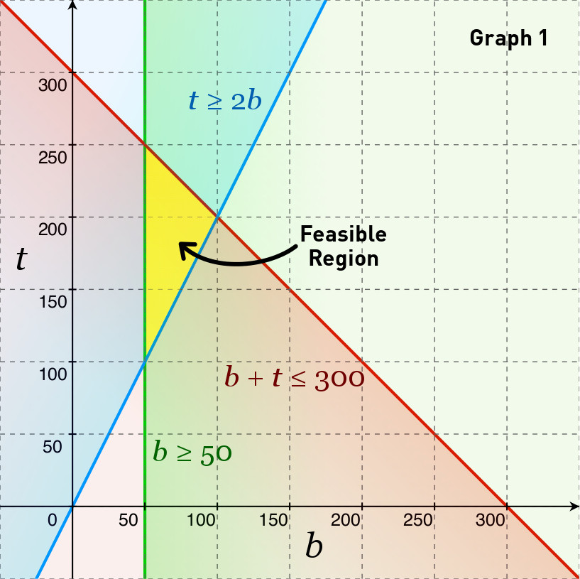
The horizontal axis is the variable b, and the vertical axis is the variable t. This example only has two variables, so we can draw a two-dimensional graph. The graph has three colored lines in it, representing our three constraints. But, our constraints are linear inequalities, which means the lines divide the graph into regions, the colored areas on the graph. (The lines and regions don't stop at the edges of the graph, they extend forever. But we are only interested in what is shown here.)
Each region indicates the possible solutions which satisfy that constraint. For example, the red region (below and to the left of the red line) indicates all the points that would satisfy the constraint b + t ≤ 300. You can pick any point in that region, and it would make that inequality true. Any point outside of the region would make that inequality false.
The three regions defined by our inequalities overlap near the middle of the graph. The region where all the constraints overlap is called the feasible region. You can choose any point in that region, and it will be a feasible solution, meaning that it makes all the inequalities true. In other words, every point in the feasible reason satisfies all of our constraints.
You may recall from earlier that we figured out three feasible solutions to our UI layout specification. We started with B being 50 pixels wide and T being 100 pixels wide; this corresponds to the point b=50, t=100 on the graph. Next we tried increasing the width of T, and arrived at the feasible solution b=50, t=250. But we decided that was not optimal, so then we tried increasing B instead, and arrived at the solution b=100, t=200, which was the optimal solution. If you look at the graph, you will notice that those three solutions are the three corners of the feasible region!
It's not a coincidence that the three feasible solutions we found, including the optimal solution, are corners of the feasible region. Linear programming theory tells us that at least one of the corners must be an optimal solution. In some systems, every point along one of the sides of the feasible region is equally optimal, including all the corners of that side. But the optimal solution must always be on the border of the feasible region. The optimal solution cannot be in the middle of the feasible region, nor outside of it.
For some systems, the feasible region goes on forever. Imagine if we did not have the red line, b + t ≤ 300. The feasible region would be the overlap of the green and blue regions, which continues upwards forever, beyond the top of the graph. Our system would be an unbounded system, and it would have no optimal solution. No matter what point you chose in the green/blue region, there are an infinite number of better solutions above and to the right of the point you chose. You could keep choosing better and better points forever, and you would never find the "best" point. (Fortunately, the Cassowary algorithm prevents a system from being unbounded, so you don't have this problem.)
For a system with only two variables, one way to solve a linear programming problem is to draw a graph like this, then check every corner of the feasible region so see which point (or points) are optimal. It is possible to use this approach for systems with three variables, although it is harder because you would need a three-dimensional graph.
But you can't really graph systems with more than three variables. And checking every single corner is not very efficient: if we had hundreds of constraints, the feasible region could have hundreds of corners to check. Besides, it would be very hard and inefficient to teach a computer to interpret a graph the way a human does, so we can't use this approach to implement UI layout constraints, anyway.
We want a technique that will work no matter how many variables we have, and will perform the fewest necessary calculations to find an optimal solution, and can be easily programmed into a computer. Fortunately, we have the simplex method, and its descendants like the Cassowary algorithm.
Recap
In this post, we have learned what UI layout constraints and linear programming are. We also converted an example layout constraint problem into a system of linear equations and inequalities, and graphed them visually.
In part 2 of this series (coming eventually), we will build upon this knowledge to learn about the simplex method, and use it to solve our example problem. In later parts, we will learn about the Cassowary algorithm and how to implement it in the computer.